players <- gamedata %>%
  group_by(namePlayer, idPlayer) %>%
  summarise(
    total_minutes = sum(minutes),        # Total minutes played
    avg_minutes = mean(minutes),         # Average minutes per game

    # Shooting efficiency (season totals)
    pctfg3 = sum(fg3m) / sum(fg3a),     # 3PT% (∑makes / ∑attempts)
    pctfg2 = sum(fg2m) / sum(fg2a),     # 2PT%
    pctft = sum(ftm) / sum(fta),        # FT%

    # Per-game averages
    fg3a = mean(fg3a),                  # 3PT attempts per game
    fg2a = mean(fg2a),                  # 2PT attempts per game
    fta = mean(fta),                    # FT attempts per game
    oreb = mean(oreb),                  # Offensive rebounds
    dreb = mean(dreb),                  # Defensive rebounds
    ast = mean(ast),                    # Assists
    stl = mean(stl),                    # Steals
    blk = mean(blk),                    # Blocks
    tov = mean(tov),                    # Turnovers
    pts = mean(pts)                     # Points
  ) %>%
  ungroup()
Introduction
The 2024–25 NBA season showcases basketball’s accelerating evolution beyond traditional positions. As 7-foot centers anchor offenses from the three-point line and 6’8” point guards orchestrate pick-and-rolls, conventional labels like “point guard” or “center” increasingly fail to capture players’ actual on-court impact. This positional revolution demands new analytical frameworks that reflect how players contribute rather than where they’re listed on depth charts.
To better understand the game’s fluidity, this analysis uses Principal Component Analysis (PCA) and K-Means clustering to group players based on statistical profiles rather than positional assumptions. PCA reduces complex, high-dimensional performance data into interpretable axes of variation — such as scoring efficiency vs. usage, or interior vs. perimeter tendencies — while K-Means identifies natural groupings of player archetypes within that space. Together, these methods provide a clearer lens for evaluating how NBA players truly shape the game in 2024–25.
Analytical Approach: Skill-Based Taxonomy
We confront this paradigm shift through a two-stage statistical methodology:
Dimensionality Reduction via PCA
Condenses 13 core performance metrics into fundamental skill dimensions: \[\small{\text{PC}_k = \sum_{j=1}^{p} w_{kj}X_j}\] Where \(\text{PC}_k\) represents orthogonal basketball competencies (shooting, creation, defense)Unsupervised Clustering via K-means
Groups players by skill similarity through variance minimization: \[\small{\underset{\mathcal{C}}{\arg\min} \sum_{i=1}^{k} \sum_{x \in C_i} \lVert x - \mu_i \rVert^2}\] Identifying natural groupings without positional preconceptions
Core Objective:
Identify true player archetypes in the 2024-25 season and pinpoint undervalued talent where:
\[\small\underbrace{\text{Statistical Impact}}_{\text{Archetype Value}} > \underbrace{\text{Market Perception}}_{\text{Contract/Salaries}}\]
Why Skill-Based Analysis Matters
Front offices require analytical frameworks that:
- Replace legacy positions with role-based skill profiles
- Quantify hidden value beyond box score statistics
- Exploit market inefficiencies in roster construction
- Optimize lineups through complementary skill pairings
Data
Player statistics were programmatically collected from the NBA’s official statistics database (NBA.com/stats) using the nbastatR R package. The dataset encompasses:
- Season Coverage: Complete 2024-25 regular season (October 22, 2024 - April 13, 2025)
- Collection Scope: All player-game observations for rotation players
- Automation: Scripted daily updates via NBA API
Raw Dataset Structure
- Observations: 26,306 player-game entries
- Variables: 58 metrics spanning four key dimensions
The 58 variables span four critical basketball dimensions:
\[ \begin{bmatrix} \text{Game Context} & \text{Player Metadata} & \text{Shooting Splits} & \text{Box Score Metrics} \\ \color{#6c757d}{\small\text{(date, matchup)}} & \color{#6c757d}{\small\text{(name, ID, position)}} & \color{#6c757d}{\small\text{(FG2M/A, FG3M/A, FTM/A)}} & \color{#6c757d}{\small\text{(PTS, REB, AST, STL, BLK, TOV)}} \end{bmatrix} \]
From Game Logs to Player Profiles
To analyze player performance at a season level, the raw game-level dataset was aggregated into player-season statistics using dplyr in R. This transformation condenses granular game-by-game performance into interpretable season-level metrics, enabling player profiling and clustering analyses.
These aggregated profiles form the foundation for subsequent PCA and clustering analyses to identify distinct player archetypes.
Key Engineering Decisions
Shooting Efficiency Calculation
Uses season totals rather than game averages:
\[
\text{pctfg3} = \frac{\sum \text{fg3m}}{\sum \text{fg3a}}
\]
Why? More stable than \(\text{mean(pctFG3)}\) which overweights outlier games.
Rebound Separation
Distinct oreb (offensive) and dreb (defensive) instead of total rebounds:
oreb→ Second-chance creation
dreb→ Defensive cleanup
Shot Spectrum
Separate tracking of perimeter and interior attempts:
- Perimeter:
fg3a(3PT attempts)
- Interior:
fg2a(2PT attempts)
Player Minutes Distribution
The histogram below in Figure 1 shows the distribution of total_minutes played during the 2024-25 NBA season:
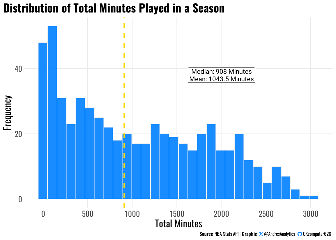
Distribution Characteristics
The histogram in Figure 1 reveals a right-skewed distribution of total minutes played:
- Median: \(908\) minutes
- Mean: \(1043.5\) minutes
- Skewness: \(\text{mean} > \text{median}\) indicates positive skew
Data Preprocessing Pipeline
Based on the minutes distribution and analytical objectives, we implement two key preprocessing steps:
- Player Filtering:
- Retain only rotation players with ≥900 minutes played
- Ensures meaningful skill pattern analysis
- Removes deep bench/garbage time players
- Retain only rotation players with ≥900 minutes played
- Feature Selection:
- Remove
total_minutes(filtering criterion only)
- Exclude non-skill columns (player names, IDs, etc.)
- Retain only performance metrics relevant to archetype analysis
- Remove
Preprocessing Outcomes
- Players retained: 288 (rotation players meeting minutes threshold)
- Features processed: 13 (13 skill metrics)
- Key decisions:
- Filtered out 281 players below minutes threshold
- Removed
total_minutesand other non-skill columns
- Imputed 0% 3PT accuracy for 5 non-shooters
- Filtered out 281 players below minutes threshold
Final Feature Set (13 Metrics)
The selected metrics in Table 2 capture essential basketball skills for archetype analysis:
| Category | Metrics | Description |
|---|---|---|
| Scoring | pts |
Total points scored |
| Perimeter Game | fg3a, pctfg3 |
3PT attempts and percentage |
| Interior Game | fg2a, pctfg2 |
2PT attempts and percentage |
| Free Throws | fta, pctft |
FT attempts and percentage |
| Rebounding | oreb, dreb |
Offensive/defensive rebounds |
| Playmaking | ast, tov |
Assists and turnovers |
| Defense | stl, blk |
Steals and blocks |
Feature Rationale:
- Excluded
total_minutesas it was only used for filtering - Removed non-performance columns to focus analysis on on-court skills
- Retained all shooting/rebounding/playmaking/defense metrics for PCA
ptsincluded as holistic scoring measure
Our analysis rests on comprehensive performance data in Table 3:
| Component | Details | Count |
|---|---|---|
| Player Pool | All rotation players | 288 players |
| Season Coverage | Oct 2024 - Apr 2025 | 82 games |
| Metrics Collected | 13 skill dimensions | 7 categories |
| Inclusion Criteria | ≥900 minutes played | Excluded 44% of rostered players |
Next Steps: Skill Space Analysis
With the filtered player set and curated features, we proceed to:
- Standardize metrics for PCA
- Reduce dimensionality to core skill components
- Cluster players by skill similarity
Principal Component Analysis
Conceptual Foundation
Principal Component Analysis (PCA) is a dimensionality reduction technique that transforms correlated variables into a set of linearly uncorrelated principal components:
\[\small{\text{PC}_k = w_{k1}X_1 + w_{k2}X_2 + \cdots + w_{kp}X_p}\]
Where: - \(\text{PC}_k\) = Orthogonal skill dimension - \(w_{kj}\) = Weight coefficients maximizing variance capture - \(X_j\) = Original skill metrics (e.g., pts, ast, reb)
For basketball analytics, PCA helps uncover the underlying skill dimensions driving player performance.
The Critical Role of Feature Scaling
Before applying PCA, we standardize all features using z-scores:
\[ z = \frac{x - \mu}{\sigma} \]
Why Scaling is Essential
- Equal Metric Influence: Prevents high-magnitude stats (e.g., points) from dominating lower-scale stats (e.g., block %)
- Unit Variance: Ensures all features contribute equally to total variance
- Mean Centering: Aligns features to a shared origin (μ = 0)
- Covariance Stability: Ensures PCA captures real correlations, not scale artifacts
PCA Implementation & Results
We applied PCA to the standardized player dataset to extract its core performance dimensions.
Eigenvalue Analysis
The eigenvalues in Table 4 quantify each component’s explanatory power:
| Eigenvalue | Explained Variance (%) | Cumulative Variance (%) | |
|---|---|---|---|
| Dim.1 | 5.10 | 39.23 | 39.23 |
| Dim.2 | 3.60 | 27.68 | 66.91 |
| Dim.3 | 0.94 | 7.20 | 74.11 |
| Dim.4 | 0.76 | 5.84 | 79.95 |
| Dim.5 | 0.66 | 5.07 | 85.02 |
| Dim.6 | 0.49 | 3.75 | 88.77 |
| Dim.7 | 0.43 | 3.28 | 92.05 |
| Dim.8 | 0.36 | 2.75 | 94.80 |
| Dim.9 | 0.29 | 2.20 | 97.00 |
| Dim.10 | 0.16 | 1.24 | 98.24 |
| Dim.11 | 0.11 | 0.88 | 99.13 |
| Dim.12 | 0.11 | 0.83 | 99.96 |
| Dim.13 | 0.01 | 0.04 | 100.00 |
Key Findings from Eigenvalue Analysis
- Kaiser Criterion (Eigenvalue > 1):
- Only Dim.1 (5.10) and Dim.2 (3.60) exceed the threshold
- These two components account for 66.91% of the total variance
- They represent the core performance dimensions in NBA player data
- Only Dim.1 (5.10) and Dim.2 (3.60) exceed the threshold
- Meaningful Dimensions:
- Dim.3 (0.94) and Dim.4 (0.76) are borderline significant
- The top four components capture 79.95% of total variance
- Together, they provide a more complete picture of performance variation
- Dim.3 (0.94) and Dim.4 (0.76) are borderline significant
- Diminishing Returns:
- Components beyond Dim.4 each explain <6% variance
- Cumulative variance plateaus after Dim.6 (88.77%)
- Components 7–13 likely reflect noise or redundant information
- Components beyond Dim.4 each explain <6% variance
Interpretation Summary
| Component Range | Variance Captured | Analytical Value |
|---|---|---|
| Core Dimensions (1-2) | 66.91% | Essential for analysis |
| Supplementary (3-4) | 13.04% | Important context |
| Marginal (5-13) | 20.05% | Limited value |
Strategic Implications:
- Using the top 4 components strikes a strong balance between dimensionality reduction and information retention (79.95%)
- These components shown in Table 5 form the basis for clustering players into data-driven performance archetypes
- Omitting components beyond Dim.4 avoids overfitting and reduces noise without sacrificing key insights
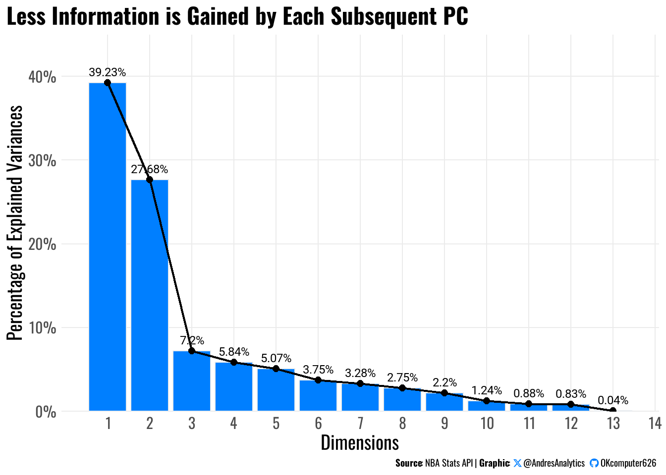
This scree plot in Figure 2 clearly illustrates how much each principal component contributes to explaining variance in NBA player performance data. The first component (PC1) accounts for 39.23% of variance, likely representing core offensive skills like scoring. PC2 explains 27.68%, probably reflecting secondary skills such as playmaking and defense. Together, these first two components capture 66.91% of the total variance - the majority of what differentiates players. The next two components (PC3 at 7.2% and PC4 at 5.84%) add some additional explanatory power, likely covering specialized skills like three-point shooting. Beyond PC4, each subsequent component contributes less than 4% of variance, with the last few components (PC5-PC10) each explaining less than 3% - essentially statistical noise that doesn’t meaningfully impact player evaluation. This pattern shows that NBA teams can effectively analyze players using just the first 2-4 principal components while still capturing nearly 80% of the relevant performance variance, allowing them to focus on the most impactful skills and ignore minor statistical fluctuations.
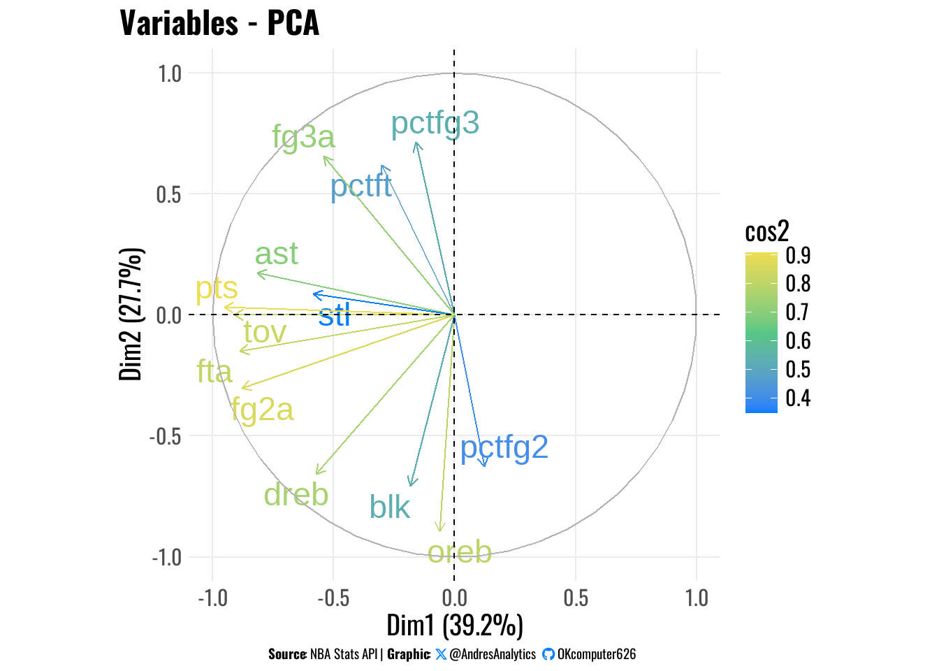
The PCA analysis in Figure 3 reveals how different NBA performance metrics contribute to principal components. Three-point shooting variables (fg3a and pctfg3) show strong loadings, reflecting their growing importance in modern basketball. Playmaking and defensive metrics (ast and stl) cluster together, indicating their combined impact on player value. Interior efficiency (pctfg2) emerges as a distinct but less dominant skill dimension. The cosine squared (cos2) values help assess how well each variable is represented in the component space. The first principal component (Dim1) explains 39.2% of total variance and is primarily driven by three-point shooting metrics, with secondary contributions from assists and steals. This pattern confirms the NBA’s evolution toward perimeter-oriented skills as the primary differentiator of player value, while still acknowledging the importance of two-way playmaking and defensive abilities.
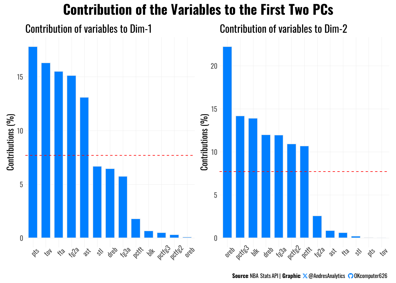
The image in Figure 4 shows the percentage contributions of different NBA statistics (variables) to the first principal component (Dim-1) in a Principal Component Analysis (PCA). The tallest bars represent the variables that contribute the most to Dim-1, meaning they have the strongest influence in defining this dimension. For example, if “Points Per Game” or “Assists” were labeled, a high contribution would suggest they are key factors driving patterns in the data. Since Dim-2 is not shown, further interpretation (e.g., trade-offs between variables) would require the full graphic.
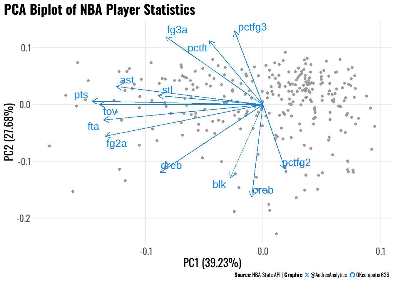
The PCA biplot in Figure 5 reveals that points (pts), assists (ast), and three-point percentage (pctfg3) are among the most influential variables on the first principal component (PC1), which alone explains 39.23% of the total variance in the dataset. These variables are commonly associated with offensive creation and scoring efficiency, suggesting that PC1 likely represents a composite axis of offensive productivity.
Players located near these vectors are likely to be high-scoring guards or wings who contribute efficiently either as shooters or facilitators. In contrast, those closer to variables like turnovers (tov) or two-point attempts (fg2a) may be more involved in interior play or exhibit less offensive efficiency — potentially high-usage, low-efficiency profiles such as slashing wings or post-heavy bigs.
While PC2 (which explains 27.68% of the variance) is not fully interpreted here, it appears to contrast perimeter skills (e.g., pctft, fg3a) with interior contributions (e.g., blk, oreb, dreb), providing a secondary axis of playstyle differentiation. Altogether, the PCA biplot enables a clearer visualization of how players group along performance-based dimensions, setting the stage for unsupervised clustering.
K-Means Clustering Analysis
Optimal Cluster Validation
1. Elbow Method
The Elbow Method evaluates the total within-cluster sum of squares (WSS) to determine the ideal number of clusters. In this analysis:
- The WSS curve shows diminishing returns starting at k = 4 or 5, where adding more clusters yields only marginal variance reduction.
- Interpretation: A 5-cluster solution balances complexity and interpretability, capturing key groupings without overfitting.
2. Silhouette Method
The Silhouette Method measures how well each player fits within its assigned cluster, based on cohesion (how close a player is to others in its cluster) and separation (how far it is from other clusters).
- The average silhouette width peaks at k = 2-3, suggesting strong, well-separated groupings at these values.
- However, despite slightly lower silhouette scores, a 5-cluster solution remains justifiable due to its richer interpretive granularity — especially in the context of diverse NBA roles and playstyles.

The 5-cluster solution in Figure 6, built on the first four principal components (capturing 79.95% of the total variance), provides both statistical robustness and basketball insight. These clusters reveal not only differences in raw production but also stylistic separation across player types — such as differentiating combo guards who score and create, from pure playmakers who facilitate without high usage. Similarly, stretch bigs are separated from rim-protecting traditional centers, reflecting spacing and interior roles.
Each cluster exhibits a unique blend of contributions across the four PCA dimensions, enabling analysts and teams to identify undervalued archetypes, compare similar players across contexts, or scout for specific stylistic needs. This approach highlights how dimensionality reduction and unsupervised learning can uncover the nuanced structure of NBA performance data beyond surface-level stats or listed positions.
PCA and K-Means Clusters
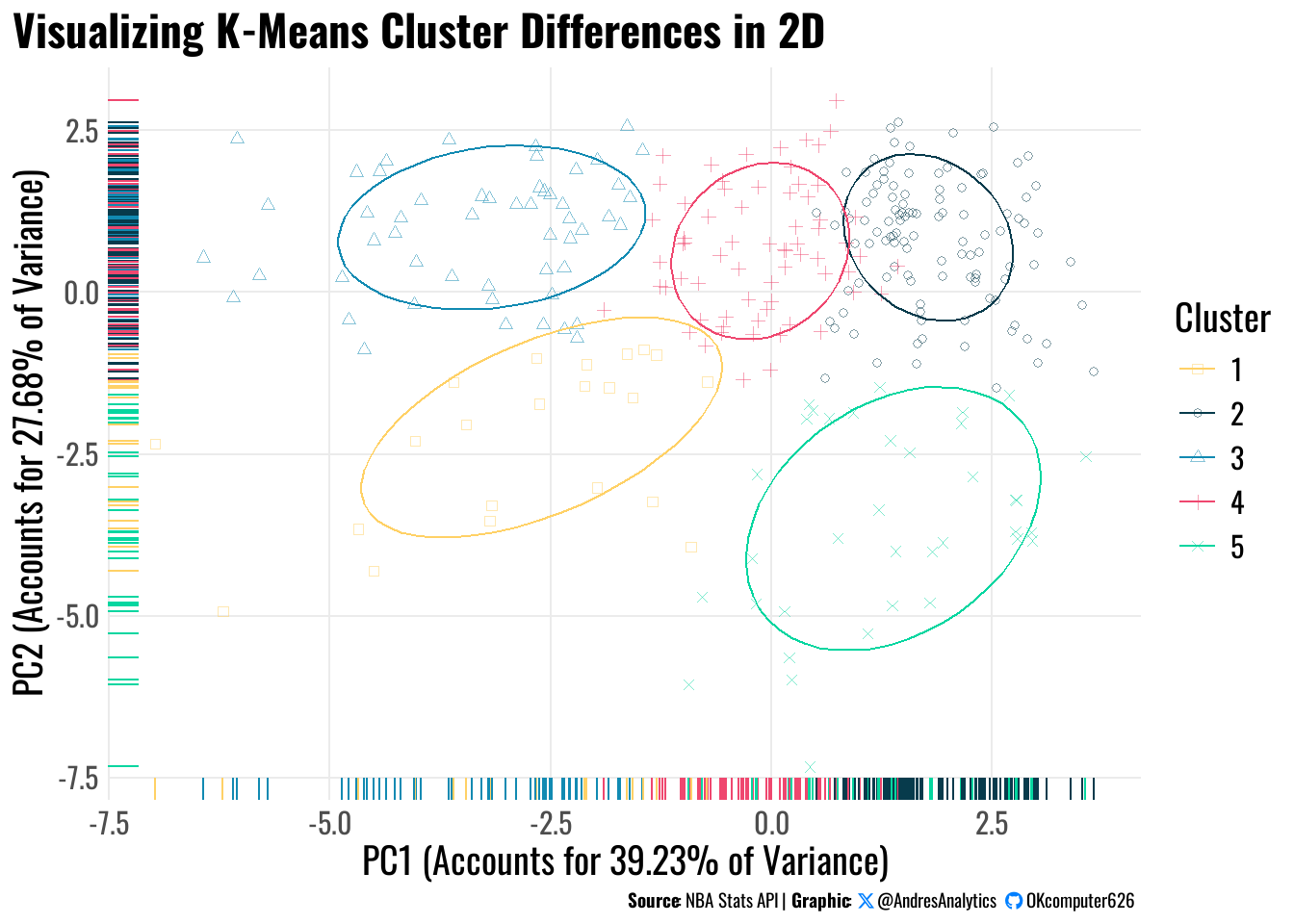
The figure below in Figure 7 illustrates the five identified clusters projected onto the first two principal components:
Interpretation Summary
This PCA plot in Figure 7 visualizes the five K-Means clusters projected onto the first two principal components:
- PC1 (x-axis) explains 39.23% of total variance, representing a dimension largely driven by offensive production and efficiency.
- PC2 (y-axis) explains 27.68% of total variance, capturing a dimension contrasting perimeter-oriented skills with interior-focused contributions.
Cluster Insights
Cluster 1 – Versatile Contributors
Positioned in the lower-left quadrant, indicating players with low offensive efficiency and limited perimeter involvement. Likely traditional bigs or low-usage interior players.
Cluster 2 – Low-Usage Role Players
Located in the upper-right quadrant. Represents balanced or efficient scorers with strong perimeter contributions, such as versatile forwards or efficient guards.
Cluster 3 – Perimeter-Oriented Shooters
Upper-left quadrant, suggesting high perimeter involvement but lower efficiency. Likely volume shooters or ball-dominant guards with streaky performance.
Cluster 4 – Balanced Average Players
Centered slightly to the right, indicating balanced players with moderate efficiency and versatile contributions across roles.
Cluster 5 – Efficient Finishers / Interior Specialists
Lower-right quadrant, representing players with high offensive efficiency and strong interior presence, such as efficient finishers or rim-running bigs.
Standardized Feature Profiles Across NBA Player Clusters
Interpretation Summary
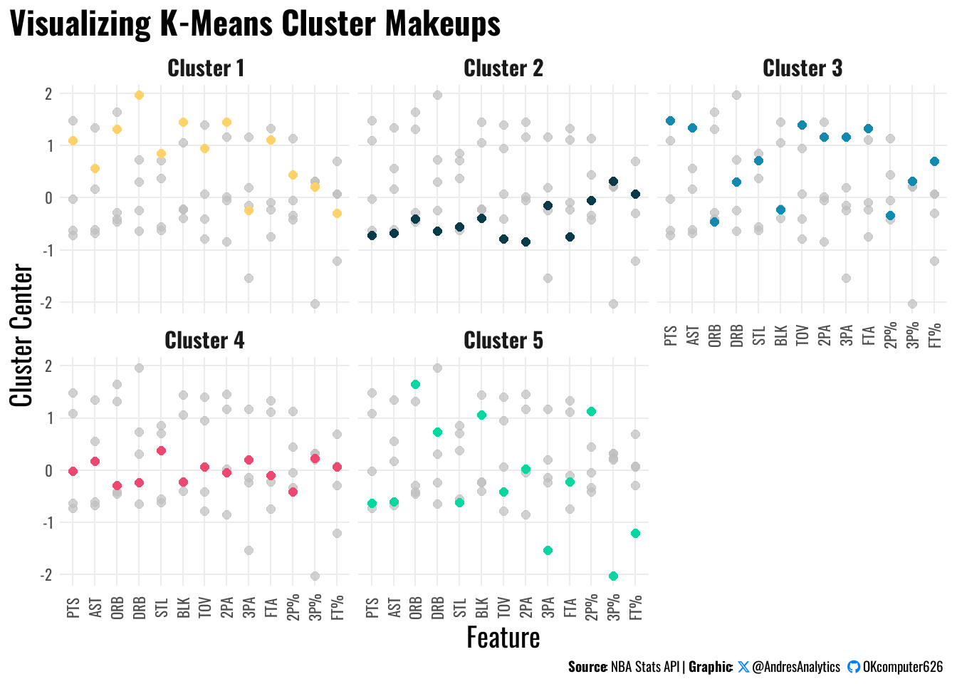
This visualization in Figure 8 displays the standardized cluster centers across key features for each of the five K-Means clusters:
- Y-axis: Cluster center value (standardized).
- X-axis: Features such as PTS, AST, ORB, DRB, STL, BLK, TOV, 2PA, 3PA, FTA, 2P%, 3P%, FT%.
Cluster Insights
Cluster 1 – Versatile Contributors
Shows strong positive values across multiple features, suggesting players who contribute in scoring, playmaking, rebounding, and defense. Likely high-usage, well-rounded players impacting many facets of the game.
Example players: Nikola Jokić, Giannis Antetokounmpo
Cluster 2 – Low-Usage Role Players
Displays negative or near-zero standardized values across most features, indicating players with minimal offensive and defensive impact. Often used in niche roles with limited involvement.
Example players: Payton Pritchard, Keegan Murray
Cluster 3 – Perimeter-Oriented Shooters
Shows high standardized values in perimeter shooting and attempts (3PA, 3P%) but average or below-average contributions in other areas. Represents players focusing on spacing and shooting from deep.
Example players: Shai Gilgeous-Alexander, Anthony Edwards
Cluster 4 – Balanced Average Players
Cluster center values hover near zero across features, indicating balanced players with moderate contributions without specific standout strengths or weaknesses.
Example players: Andrew Wiggins, Lauri Markkanen
Cluster 5 – Efficient Finishers / Interior Specialists
Displays strong positive standardized values in interior scoring efficiency (2P%) and rebounding metrics (ORB, DRB), suggesting players who finish efficiently around the rim and contribute on the boards, such as rim-running bigs or interior finishers.
Example players: Mark Williams, Deandre Ayton
Cluster Profiles Summary
The table below in Table 6 summarizes the per-game statistical averages for each identified cluster, providing further context on their typical playing time and production. This includes key metrics such as minutes per game, points, assists, rebounds, and shooting attempts, highlighting how each cluster contributes differently on the court.
One notable finding in Table 6 is that while Cluster 3 (Perimeter-Oriented Shooters) averages the highest points per game (22.02 PPG) and minutes, their offensive rebounds (0.8 ORPG) remain the lowest among clusters, reflecting their tendency to operate on the perimeter rather than attacking the glass. In contrast, Cluster 5 (Efficient Finishers / Interior Specialists) plays fewer minutes on average (22.64 MPG) yet contributes strong offensive rebounding (2.51 ORPG), underscoring their specialized role as interior scorers and rebounders despite lower scoring volume overall.
NBA Player Archetypes by Scoring and Defensive Impact (2024–25)

Interpretation Summary
This scatter plot in Figure 9 visualizes NBA players by their points per game (x-axis) and defensive contributions (y-axis), categorizing them into functionally meaningful clusters:
- X-axis: Points per game, indicating offensive scoring output.
- Y-axis: Defensive contributions (rebounds + steals + blocks), indicating defensive impact.
Cluster Insights
Efficient Finishers / Interior Specialists
Players with high defensive contributions and strong interior scoring efficiency, often including rim protectors, offensive rebounders, and finishers around the basket.
Versatile Contributors
Players with both high scoring and defensive impact, representing well-rounded stars who contribute significantly on both ends of the floor.
Low-Usage Role Players
Players with lower scoring and defensive metrics, often occupying limited roles focused on niche tasks or floor spacing without high usage rates.
Balanced Average Players
Players with moderate scoring and defensive contributions, offering balanced production across multiple areas without being extreme outliers.
Perimeter-Oriented Shooters
Players with high scoring output, particularly from perimeter shooting, but lower defensive contributions, often including ball-dominant guards and wing scorers focused on offensive creation.
Conclusion
This analysis leveraged PCA and K-Means clustering to uncover data-driven NBA player archetypes based on season-level performance metrics. By moving beyond traditional position labels, we identified nuanced skill-based clusters ranging from versatile contributors to perimeter shooters and interior specialists. These insights provide a deeper understanding of how players shape the game in the modern NBA and offer practical applications for scouting, roster construction, and strategic planning.
Future work could integrate advanced defensive metrics or tracking data to further refine these archetypes and evaluate their impact on team success.
Acknowledgements
Thank you to Alex Stern for the insightful hoopDown tutorials that guided parts of this analysis, and to Alex Bresler for developing the nbastatR package, which enabled efficient data retrieval. I also want to thank the broader R community for its extensive resources and support, and California State University, Long Beach (CSULB) for providing an academic environment that fosters analytical growth and applied learning.
This project would not have been possible without these contributions.
References
NBA Advanced Stats. (2025). Retrieved from https://www.nba.com/stats
Stern, A. hoopDown: Modern NBA analysis with R. Retrieved from https://alexcstern.github.io/hoopDown.html
Bresler, A. nbastatR: R Interface to NBA Statistics API. Retrieved from https://github.com/abresler/nbastatR